The purpose of this small project is to perform a basic sentiment analysis on the “Global indicator framework for the Sustainable Development Goals and targets of the 2030 Agenda for Sustainable Development” of United Nations. Original source file and edited version for analysis in these links to have a look how it looks like.
In the end, in perspective of wording and emotional representation of these words, we may have an insight about overall feeling of a sustainable development target document.
Indicators Analysis
This analysis is about the word counts for social indicators defined in the given data.
Hide / show the code
# Loading the libraries-----------------------------------------------------if (!require("pacman")) install.packages("pacman")p_load(pacman, readxl, RColorBrewer, tidytext, tidyverse, textdata, wordcloud)# Loading the Data----------------------------------------------------------dataset.df <-read_excel("./data/indicators.xlsx")#--------------------------------------------------------------------------
There is no added value of meaningless words such as “a,to, at etc.”. Yet, they can take a big part in our analysis. Fortunately, there are already defined dictionaries for these words. However, in our data, there could be some abbreviations or different words which is repeated but not adding any value. In our case, there are words like “IHI” or “ICH” in our data which I will define as custom word to eliminate.
Hide / show the code
custom_stop_words <-tribble(# Column names begins with ~ in the tribbles~word, ~lexicon,# Add whatever words you want to add to the initial dictionary"ii", "CUSTOM","ics", "CUSTOM","ihi", "CUSTOM","iii", "CUSTOM")# Bind the custom stop words to stop_wordsstop_words_customized <- stop_words %>%rbind(custom_stop_words)
Cleaning the Words and Removing Stop Words
The last step before we have a look on our word pool is to remove the stop words and white spaces before or after the words. 🧹
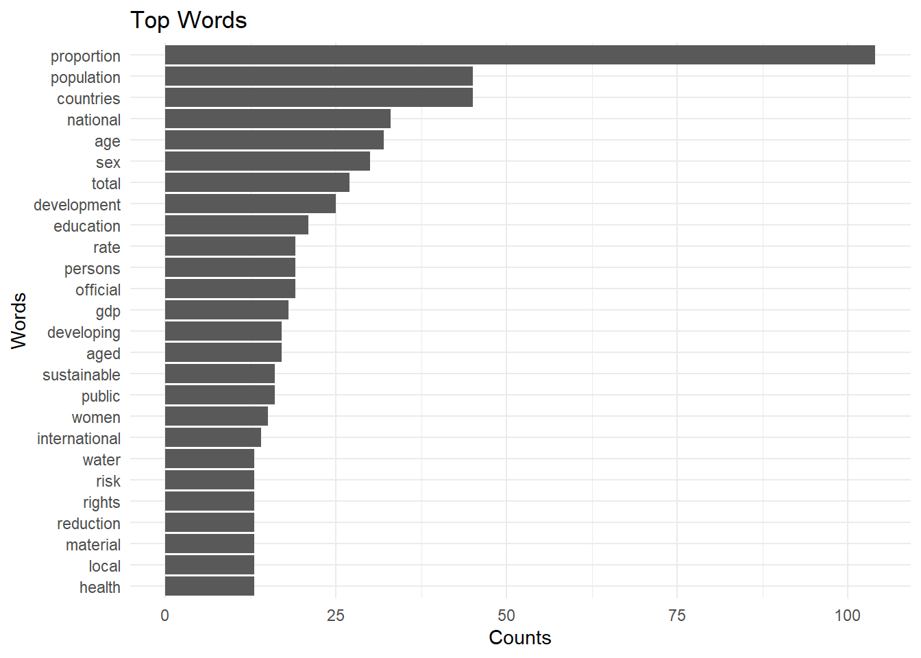
Now we cleaned the data and here are the top words: 🔝
Hide / show the code
# Getting the countstokenized_counts <- tokenized_data_cleaned %>%count(word) %>%arrange(desc(n))# Show top n words in column charttopWords <- tokenized_counts %>%slice_max(n, n =20)ggplot(topWords, aes(y=fct_reorder(word,n), x = n)) +geom_col() +theme_minimal() +labs(y ="Words", x ="Counts", title ="Top Words")
Creating Word Cloud
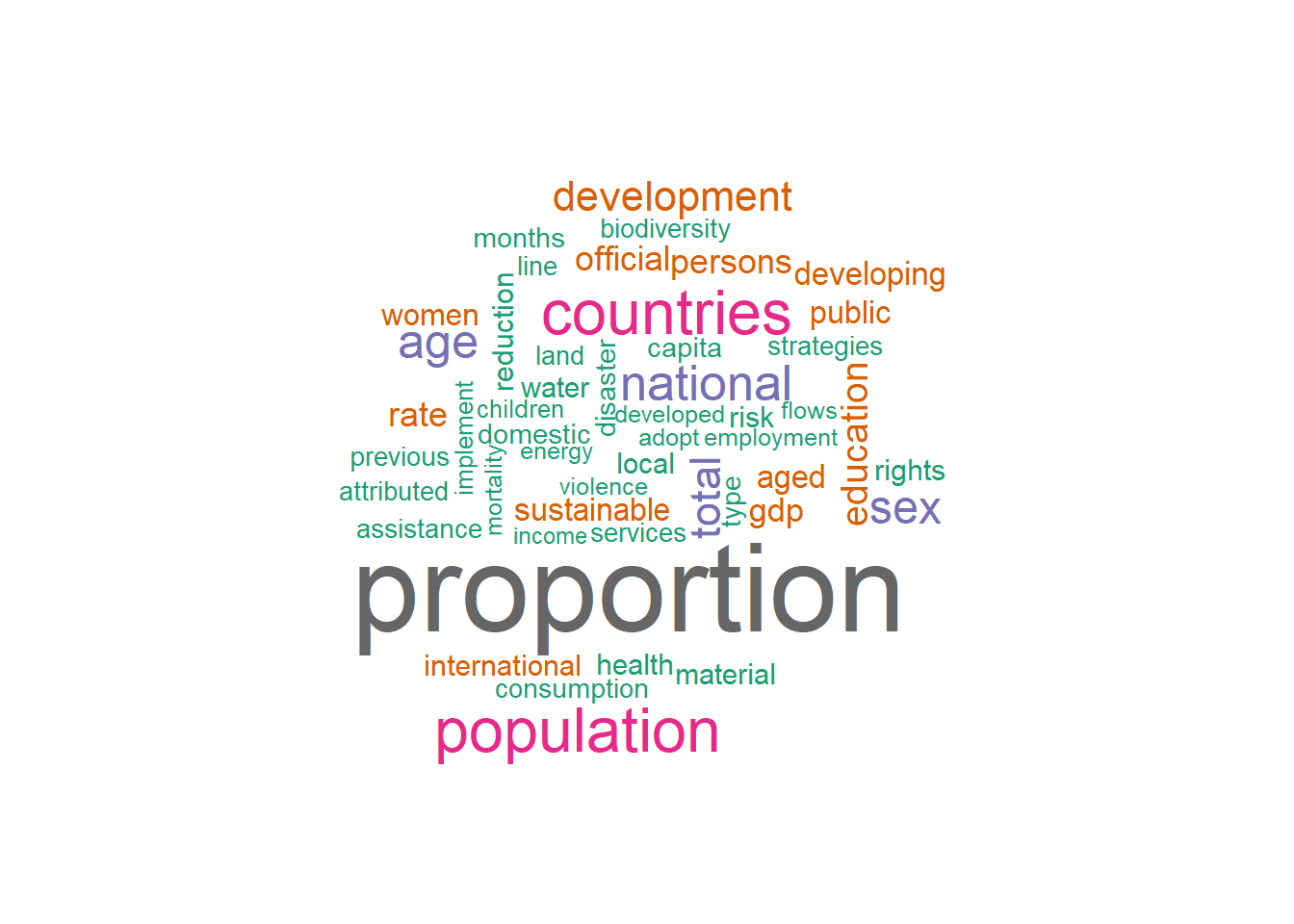
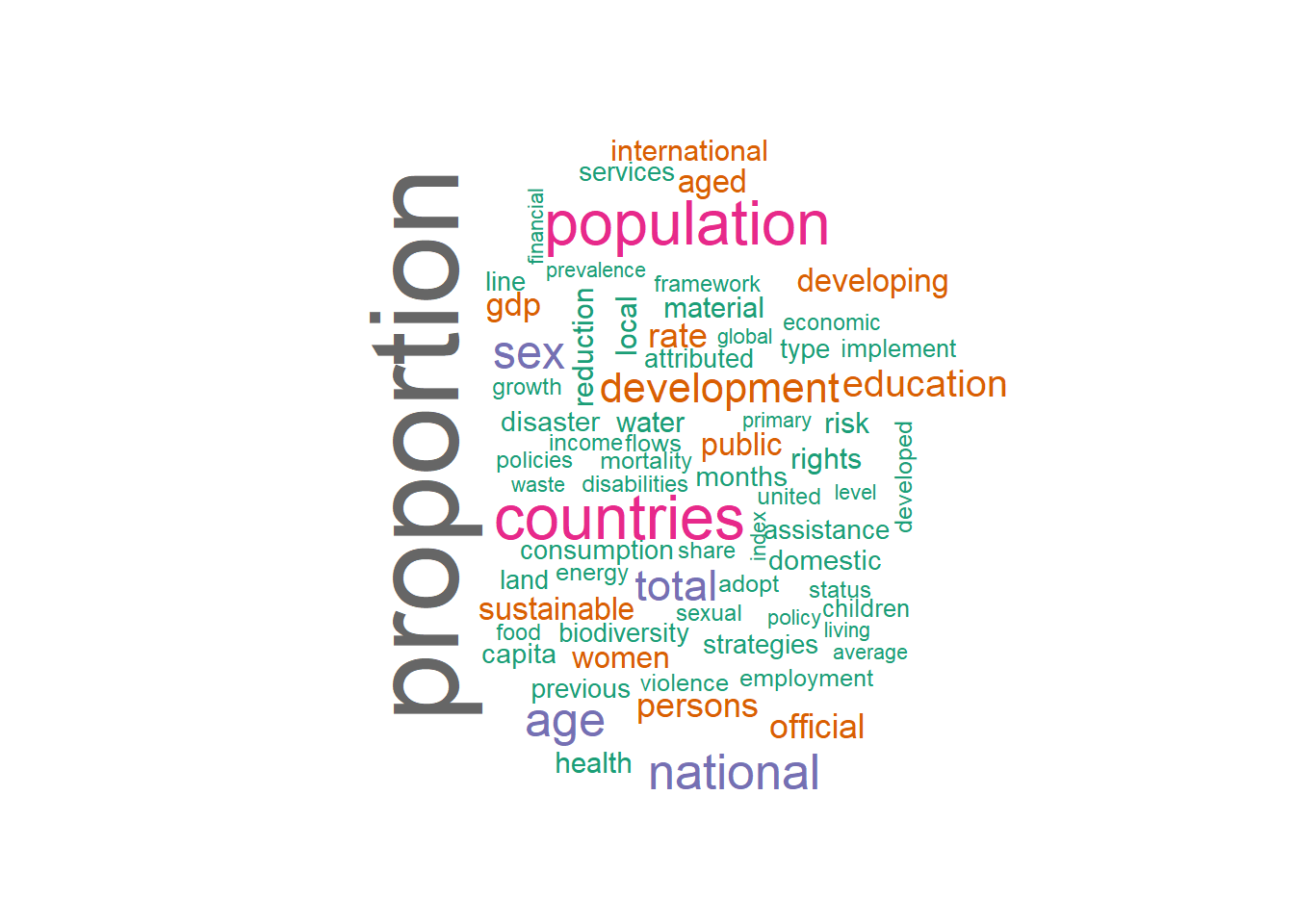
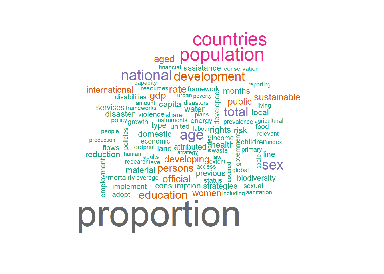
Since we have the counts of the words, we can turn them to a nicer view of a word cloud! ☁️ Our word cloud is made for top 50 – 70 – 100 words in 3 graphs in 3 different tabs below. 3️⃣
Hide / show the code
# Define your color palette from RColorBrewer# Select a palette from RColorBrewer, e.g., "Set2" with 8 colorsmy_palette <-brewer.pal(8, "Dark2") # Define a seed to freeze thingsset.seed(42)
# Create the word cloudwordcloud(words = tokenized_counts$word, # Select the column containing the wordsfreq = tokenized_counts$n, # Select the column containing the word frequencies or countsmax.words =50, # Maximum number of words to show on the graphcolors = my_palette # Use your custom color palette)
Hide / show the code
# Create the word cloudwordcloud(words = tokenized_counts$word, # Select the column containing the wordsfreq = tokenized_counts$n, # Select the column containing the word frequencies or countsmax.words =70, # Maximum number of words to show on the graphcolors = my_palette # Use your custom color palette)
Hide / show the code
# Create the word cloudwordcloud(words = tokenized_counts$word, # Select the column containing the wordsfreq = tokenized_counts$n, # Select the column containing the word frequencies or countsmax.words =100, # Maximum number of words to show on the graphcolors = my_palette # Use your custom color palette)
Sentiment Analysis
Now it’s time to make the sentiment analsis on these words. With this analysis, we matched the emotions related to these words, using NRC dictionary: 📖
Hide / show the code
sentimented_data <- tokenized_counts %>%inner_join(get_sentiments("nrc"), by =join_by(word))sentiment_counts <- sentimented_data %>%count(sentiment) %>%arrange(desc(n))sentiment_counts
# A tibble: 10 × 2
   sentiment        n
   <chr>        <int>
 1 positive       121
 2 trust           75
 3 negative        70
 4 fear            46
 5 sadness         41
 6 anticipation    40
 7 anger           33
 8 joy             29
 9 disgust         26
10 surprise        11
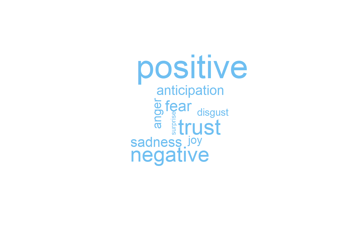
Word Cloud of Sentiments
Here is the result for 10 emotions listed in this dictionary:
As it can be seen, sustainable targets by UN document filled with mostly positive emotions and trust!
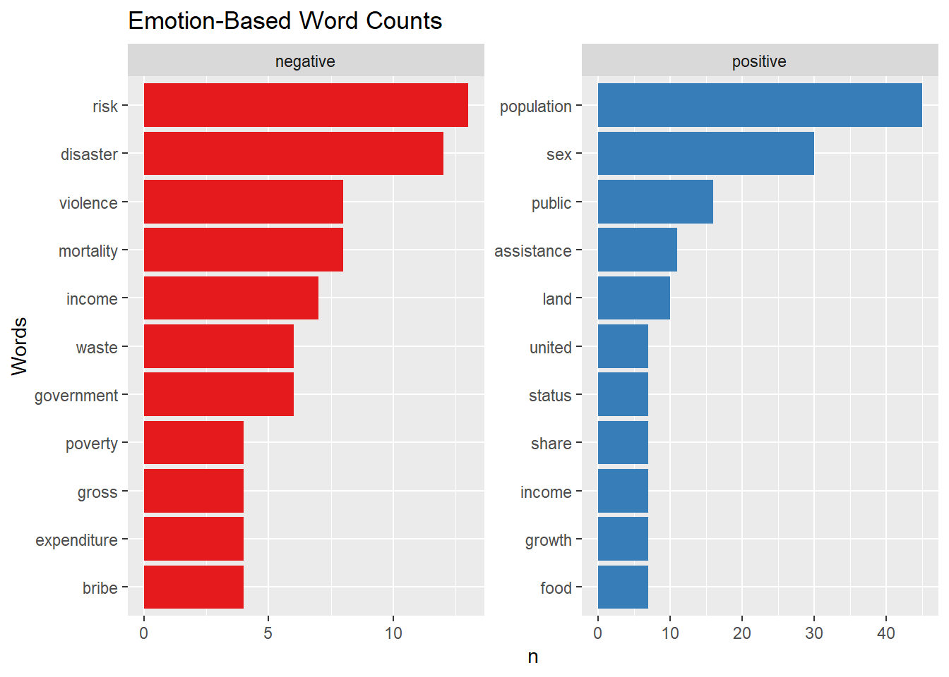
Emotion-Based Word Counts with NRC Dictionary
Finally, we can also drill down and see which words led us here. In below, we calculate the top words based on their emotional link for specifically 2 emotion categories as “positive” & “negative”.
Hide / show the code
sentimented_counts <- sentimented_data %>%# Filtering the desired sentimentsfilter(sentiment %in%c("positive", "negative")) %>%# Grouping by sentiment to find after top 3 words for each sentimentgroup_by(sentiment) %>%# Getting the top 3 sentimentslice_max(n, n=10) %>%# Clear groupingungroup() %>%# Create a factor called word_factor that has each word ordered by the countmutate(word_factor =fct_reorder(word,n))print(sentimented_counts, n=30)
# A tibble: 22 × 4
   word            n sentiment word_factor
   <chr>       <int> <chr>     <fct>
 1 risk           13 negative  risk
 2 disaster       12 negative  disaster
 3 mortality       8 negative  mortality
 4 violence        8 negative  violence
 5 income          7 negative  income
 6 government      6 negative  government
 7 waste           6 negative  waste
 8 bribe           4 negative  bribe
 9 expenditure     4 negative  expenditure
10 gross           4 negative  gross
11 poverty         4 negative  poverty
12 population     45 positive  population
13 sex            30 positive  sex
14 public         16 positive  public
15 assistance     11 positive  assistance
16 land           10 positive  land
17 food            7 positive  food
18 growth          7 positive  growth
19 income          7 positive  income
20 share           7 positive  share
21 status          7 positive  status
22 united          7 positive  united
Hide / show the code
my_palette2 <-brewer.pal(8, "Set1") ggplot(sentimented_counts, aes(x = word_factor, y = n, fill = sentiment)) +geom_col(show.legend =FALSE) +facet_wrap(~ sentiment, scales ="free") +coord_flip() +labs(title ="Emotion-Based Word Counts",x ="Words") +# Let's also apply our nice colors which we used in word cloud!scale_fill_manual(values = my_palette2)
Conclusion
In this project, we performed a basic text and sentiment analysis with R and NRC dictionary to be able to see the emotions hidden the wording of sustainability targets of UN. As a result, we found that positively related words are the majority in the file even if the goals are about reducing the ‘poverty,violence, disasters, bribe’ which are negative words.
For further analysis, words can be optimized more by manually eliminating some words which have a sentiment equivalence in the dictionary but not making a lot of sense like “gross,mortality, government, united”.